Functions
Use sum, average, minimum, maximum, count, counta, round functions.
Functions help us in analyzing and referencing data. To use functions in a worksheet, first of all we need some data on which the functions are to be applied. Any function needs some arguments to be passed to it as parameters, upon which the calculations or other operations are performed.
Say we need to add the numbers present in some cells. We can use the ‘SUM’ function to perform this task. To use the ‘SUM’ function, first select the cell where you want to put the result of the addition operation. Then click on ‘Insert’ from the main menu bar, from the resulting drop-down, click on ‘Function’. This opens the ‘Function Wizard’. All this has been shown below.
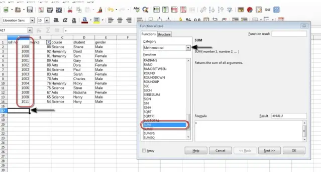
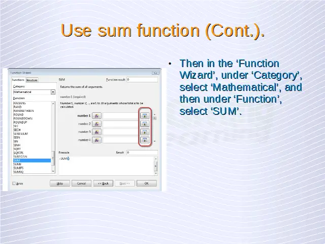
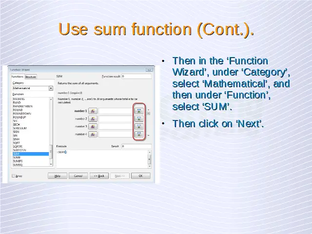
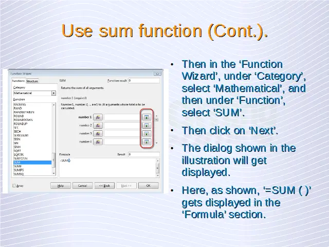
The selected cell is the one where the sum of the cell values which have been highlighted needs to be put in. Then in the ‘Function Wizard’, under ‘Category’, select ‘Mathematical’, and then under ‘Function’, select ‘SUM’. Then click on ‘Next’. The below shown dialog will get displayed.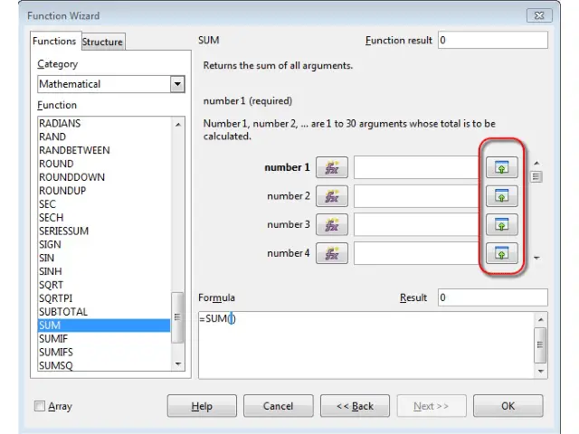
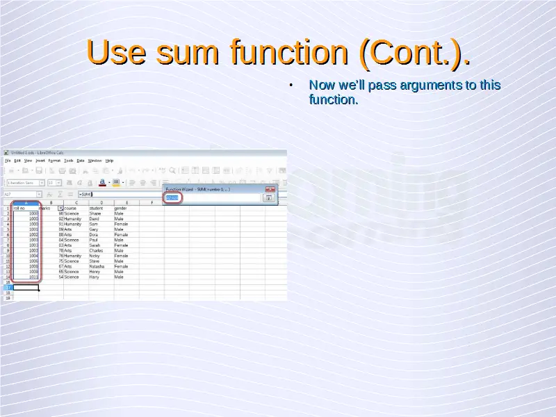
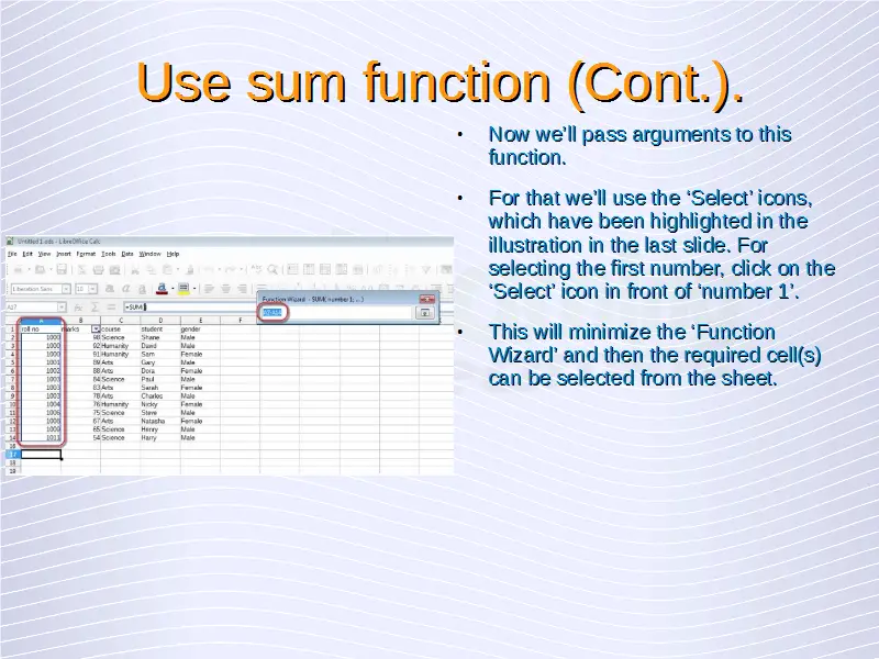
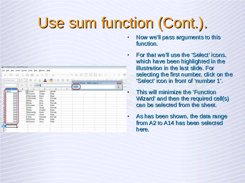
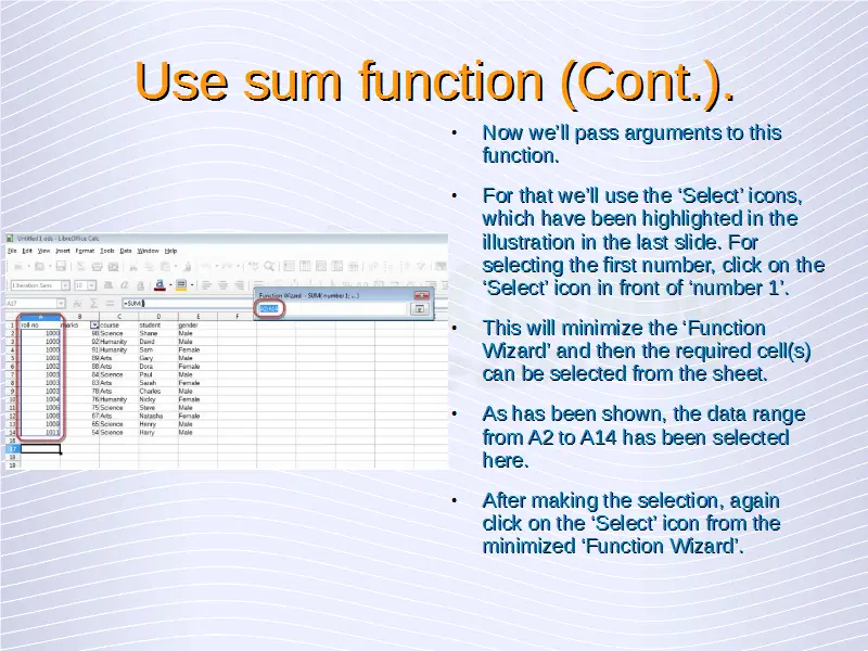
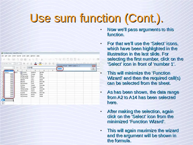
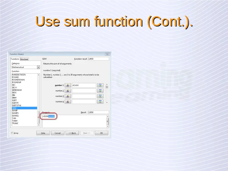
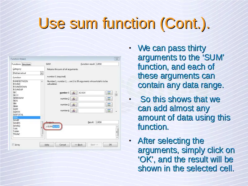
Here, as shown, ‘=SUM ( )’ gets displayed in the ‘Formula’ section. Now we’ll pass arguments to this function. For that we’ll use the ‘Select’ icons, which have been highlighted above. For selecting the first number, click on the ‘Select’ icon in front of ‘number 1’. This will minimize the ‘Function Wizard’ and then the required cell(s) can be selected from the sheet.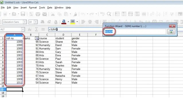
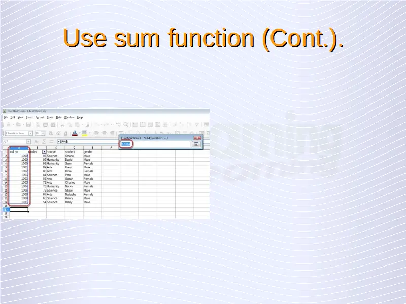
As has been shown above, the data range from A2 to A14 has been selected here. After making the selection, again click on the ‘Select’ icon from the minimized ‘Function Wizard’. This will again maximize the wizard and the argument will be shown in the formula.
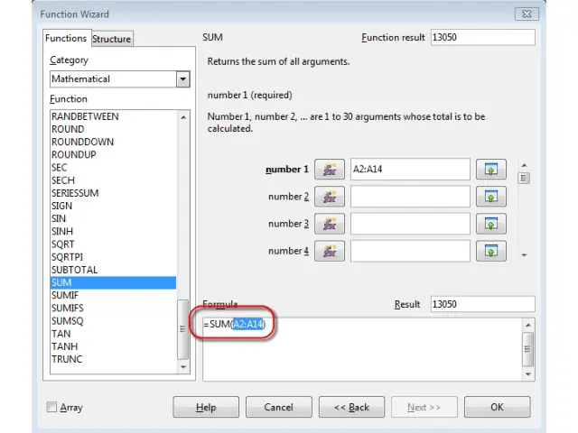
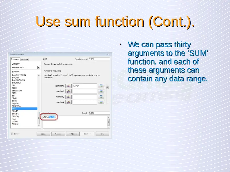
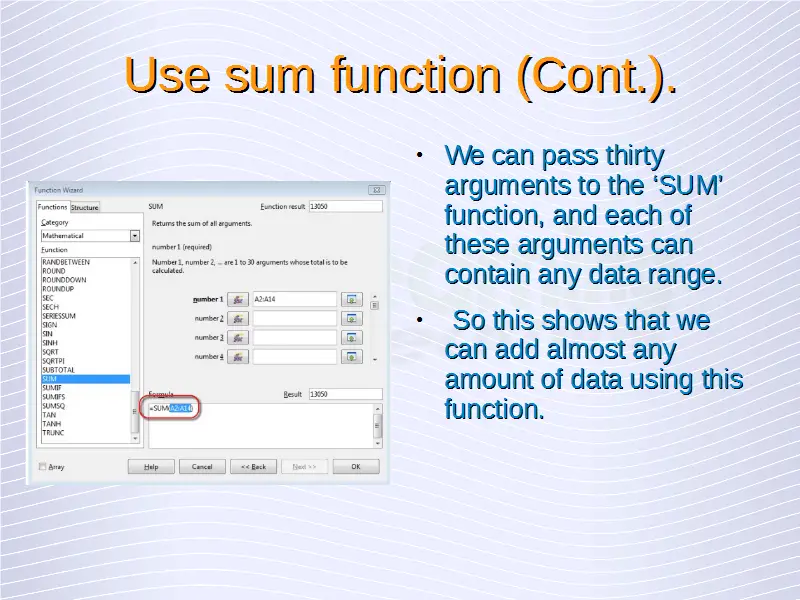
We can pass thirty arguments to the ‘SUM’ function, and each of these arguments can contain any data range. So this shows that we can add almost any amount of data using this function. After selecting the arguments, simply click on ‘OK’, and the result will be shown in the selected cell.
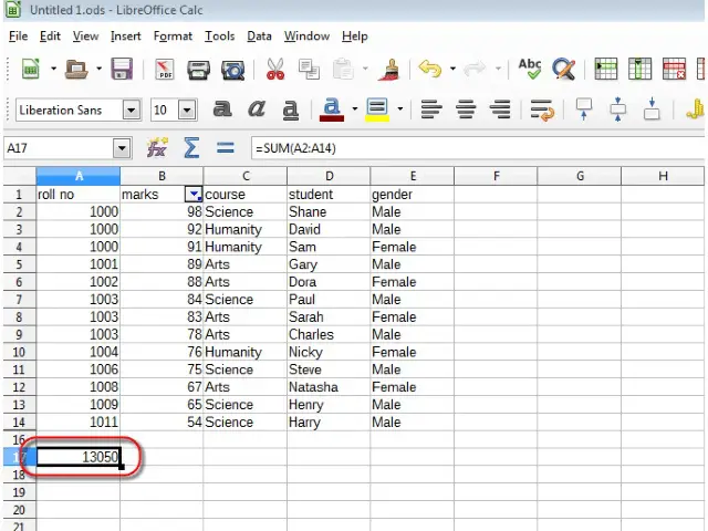
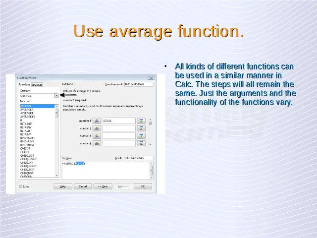
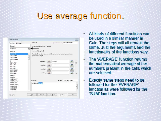
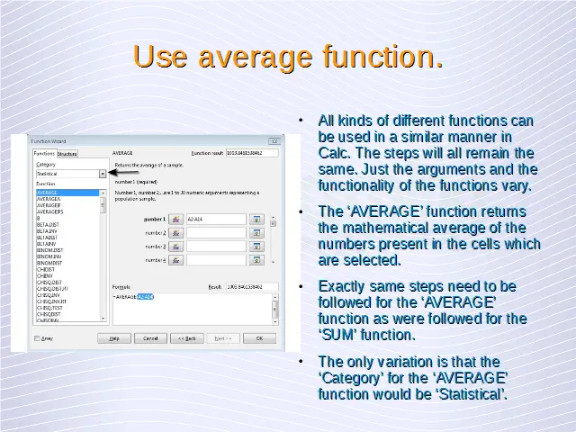
All kinds of different functions can be used in a similar manner in Calc. The steps will all remain the same. Just the arguments and the functionality of the functions vary.
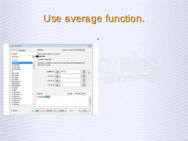
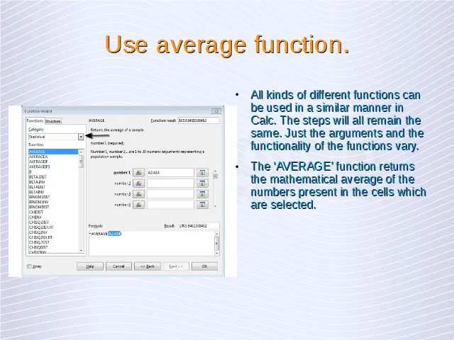
The ‘AVERAGE’ function returns the mathematical average of the numbers present in the cells which are selected. Exactly same steps need to be followed for the ‘AVERAGE’ function as were followed for the ‘SUM’ function. The only variation is that the ‘Category’ for the ‘AVERAGE’ function would be ‘Statistical’.
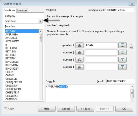
To get the minimum and maximum values from any list of arguments, we can use the ‘MIN’ and ‘MAX’ functions from the ‘Statistical’ category respectively.
The ‘COUNT’ function form the ‘Statistical’ category counts how many numbers are present in the argument list. This function only counts how many numbers are present in the argument list, and ignores other types of values like text.
The ‘COUNTA’ function from the ‘Statistical’ category counts how many values are present in the argument list. This function counts the number of all kinds of values present in the argument list, be it numbers or text or any other.
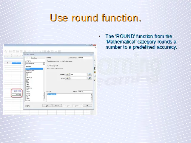
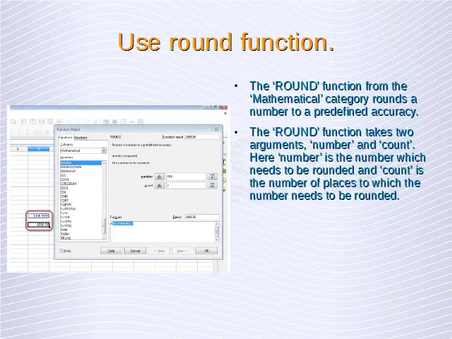
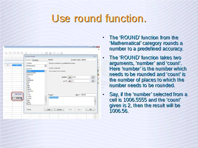
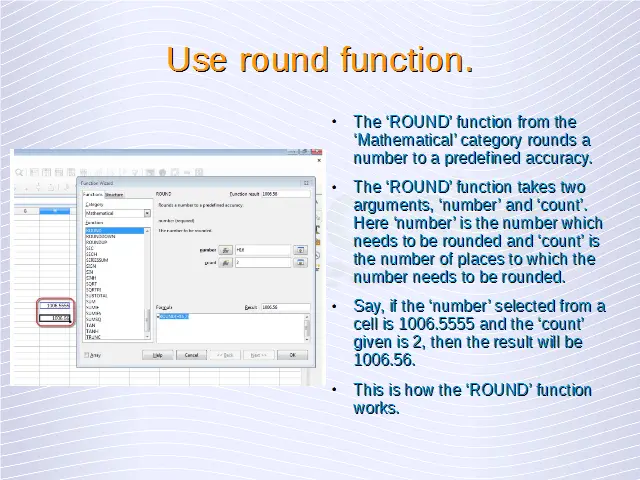
The ‘ROUND’ function from the ‘Mathematical’ category rounds a number to a predefined accuracy. The ‘ROUND’ function takes two arguments, ‘number’ and ‘count’. Here ‘number’ is the number which needs to be rounded and ‘count’ is the number of places to which the number needs to be rounded. Say, if the ‘number’ selected from a cell is 1006.5555 and the ‘count’ given is 2, then the result will be 1006.56. This is how the ‘ROUND’ function works.
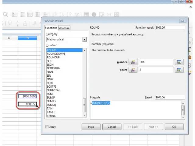
Use the logical function if (yielding one of two specific values) with comparison operator: =, >, <.
To use the logical function ‘IF’, we need to follow the same steps as above to reach the ‘Function Wizard’. In the ‘Function Wizard’, select ‘Logical’ in the ‘Category’ and from ‘Function’, select ‘IF’. Click on ‘Next’ and the following dialog is displayed.
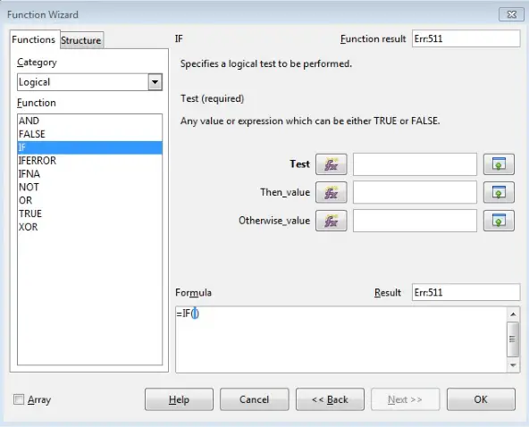
The ‘IF’ function takes three arguments, these are ‘Test’, ‘Then_value’ and ‘Otherwise_value’. ‘Test’ is the condition which needs to be tested for being either true or false. A condition could be anything and can be defined with the help of comparison operators. Here we’ll put a simple condition ‘K8>1000’, this will check whether the number present in the cell K8 is greater than 1000 or not. ‘Then_value’ defines the value which will get printed in the target cell if the condition is satisfied and ‘Otherwise_value’ defines the value which will get displayed if the condition is not satisfied. Here we’ll put the ‘Then_value’ as “Is greater than 100” and ‘Otherwise_value’ as “Is less than 1000”. Anything which is put inside “” in Calc is considered to be text by the tool, this should be kept in mind while making inputs to the tool. After making all the inputs, click on ‘OK’.
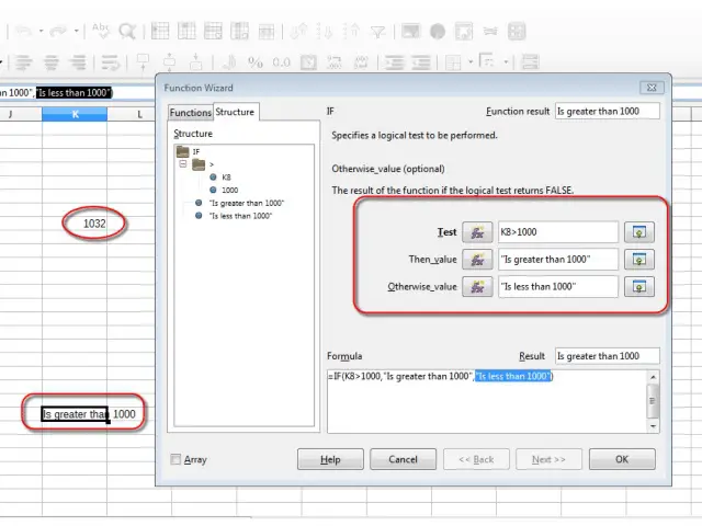
Since the value in cell K8 here is 1032, which is greater than 1000, so “Is greater than 1000” gets displayed in the selected cell. This is how ‘IF’ function works.
Related Lesson
This lesson will teach us about the various database functions available. Specifically, the DSUM function, which adds all of the cells in a data range that matches the search criteria.
Advanced Spreadsheets – Database Functions


