Advanced Spreadsheets – Using Pivot Tables
Create and modify a pivot table/data pilot.
A pivot table is a very effective and efficient tool for comparing, combining, and analyzing large amounts of data in a simple manner. To use pivot table, the first thing which is required is some raw data. The data should be in the form of a database table consisting of rows and columns. Data can be contained in a Calc spreadsheet or can be an external file or database.
When data is contained in a Calc spreadsheet in the form of a table, then the most important point is to format your data in such a way so that it can be identified as a list. You just need to select any cell within the list and the tool will automatically pick up your list based on some rules. Any empty row or column, or the upper or left border is considered as the boundary of the list. This is why it is very important to never have empty rows or columns within a list. At the same time, individual lists should be marked by a boundary of empty rows or columns.
Another point is that only one cell must be selected within the list. If more than one cell is selected, then only the particular selected cells are considered to be the whole list. The last point is that all the Calc lists must always follow the normal linear structure. All data must be entered into the same column in order to be analyzed by a pivot table.
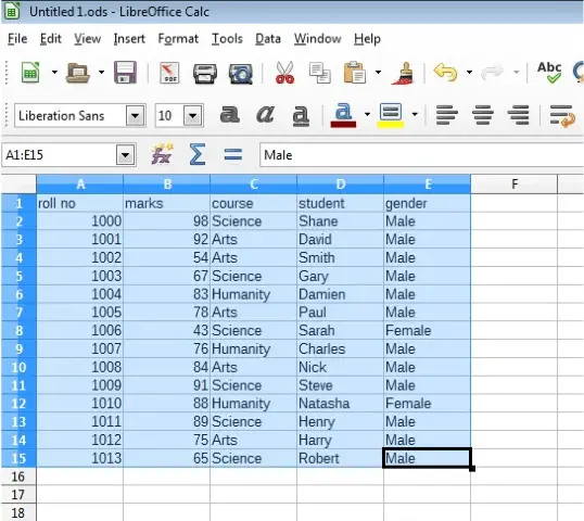
Below is a sample data table which we are going to use for this illustration.

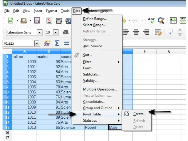
We just need to select one cell within the list. After selecting the cell, click on ‘Data’ button from the main menu bar. From the resulting drop-down, select ‘Pivot Table’ and click on ‘Create’.

From the ‘Select Source’ dialog box which appears, check ‘Current Selection’ and click on ‘OK’. This will open the ‘Pivot Table Layout’ dialog box.

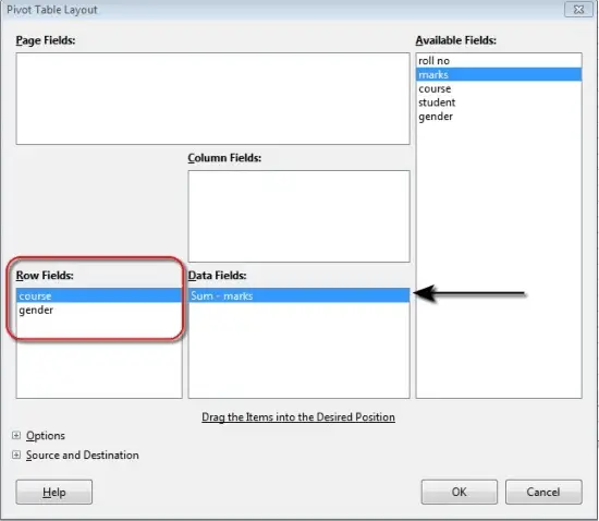
In this dialog box, we have four white areas which showcase the layout of the final result. These areas are ‘Page Fields:’, ‘Column Fields:’, ‘Row Fields:’, and ‘Data Fields:’. We also have an area called ‘Available Fields:’ which contains the names of all the data fields in our source table. We can simply drag and drop these available fields into the different areas to get the required layout for our pivot table. Similarly, any field can also be dragged back to ‘Available Fields:’ in order to remove it from the other white areas.
Here we have put the ‘course’ and ‘gender’ fields into the ‘Row Fields’ area and ‘sum’ field into the ‘Data Fields’ area. Any field we put into the ‘Data Fields’ is marked as a sum, this means that the sum of the ‘marks’ for different groupings are going to be shown in the final result. The Row Fields become the rows in the final table and Column Fields become the columns. Page Fields have the same functionality as the Column or Row Fields. The ‘Options’ and ‘Source and Destination’ fields provide some options to select the source of the data or the destination for the table, or some filtering options, and these can be chosen as per the requirements.
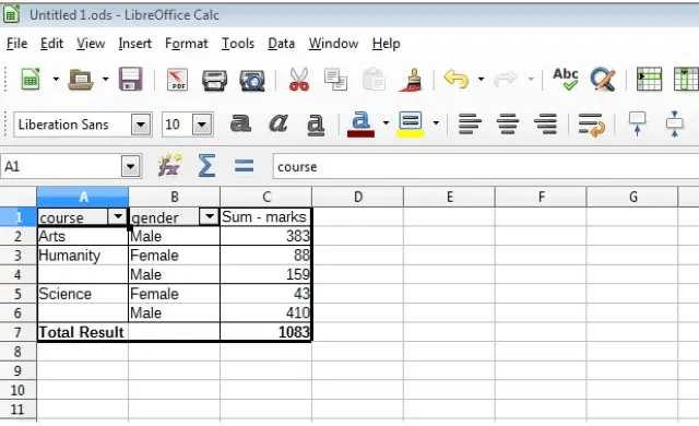
Finally, after setting all the values, click on ‘OK’. The pivot table will get generated in a new sheet or as per the destination settings.

Modify the data source and refresh the pivot table/data pilot.
If the data in the source table is modified, then it is possible to modify the pivot table to reflect these changes. After making the changes to the source table and saving them; simply go to the pivot table, right-click on the table and from the resulting shortcut menu, click on ‘Refresh’. This will update the pivot table for any changes which have been made to the source data.
But the pivot table can only be refreshed if the changes have been made to the contents and not the data labels. If the labels have been modified, then a new pivot table will have to be generated.


