Advanced Spreadsheets – Mathematical Functions

Use mathematical functions: rounddown, roundup, sumif.

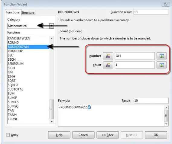
To use mathematical functions, in the same ‘Function Wizard’, select the ‘Mathematical’ category. From the ‘Function’ drop-down list, select ‘ROUNDDOWN’. This function rounds a number down to a predefined accuracy. This means that the number is rounded in such a way that the lower value is always displayed.

After selecting ‘ROUNDDOWN’, click on ‘Next’. This function will take two inputs, ‘number’ and ‘count’. ‘number’ is the number which needs to be rounded down and this can be selected from the sheet using the ‘Select’ icon. ‘count’ is the number of places down to which the number needs to be rounded. This can be entered manually or can be selected from the sheet.

After selecting everything, click on ‘OK’. This will display the result in the selected cell. As an example, if the ‘number’ selected is say ‘51.867’ and ‘count’ is given as ‘2’, then the result will be ‘51.86’.

The ‘ROUNDUP’ function is exactly similar to the ‘ROUNDDOWN’ function, with the only point of difference being that in ‘ROUNDUP’, the number is rounded up to the predefined accuracy. This simply means that in this case, the higher value is always going to be displayed. Rest everything, including the steps of usage, remain exactly same. Taking the same example, if the ‘number’ selected here is again ‘51.867’ and ‘count’ is given as ‘2’, then the result this time will be ‘51.87’. The next highest value will be taken.

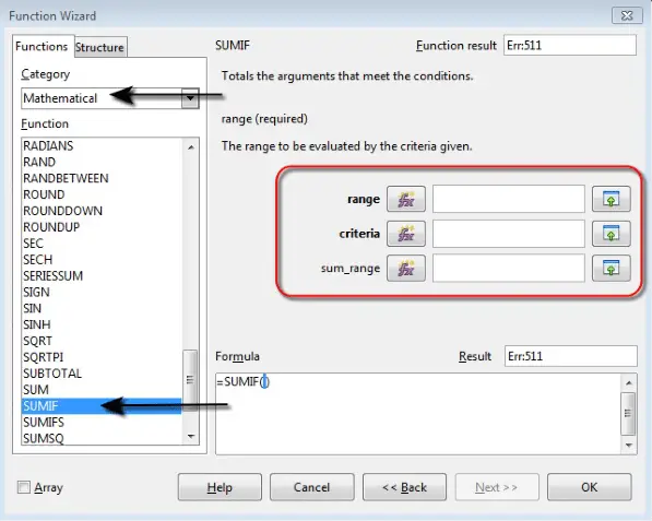
In the same wizard, we have the ‘SUMIF’ function. This function totals the arguments if they meet the specified conditions. The ‘SUMIF’ function takes three arguments, ‘range’, ‘criteria’ and ‘sum_range’. ‘range’ is the cell range which is to be evaluated by the given criteria, ‘criteria’ is the criteria which need to be applied to this range and ‘sum_range’ gives the range from which the values are to be totaled.

All these arguments can be entered either manually, or by using the ‘Select’ icon, or by using the ‘Function’ icon in front of the different options. This icon helps in entering a function as an argument for another function.

Let us take an example for the ‘SUMIF’ function. Let the ‘range’ which is selected contains 5 cells, and the values in these cells be ‘550’, ‘450’, ‘700’, ‘380’, and ‘750’. Now let us set the ‘criteria’ as “>500”. It should be remembered that when the ‘criteria’ includes any mathematical or logical operator, then it must be surrounded by double quotes. “>500” means greater than 500. So this ‘criteria’ will check the cells specified in the range and will only take those cells whose value is greater than 500. So here the selected cells will be ‘550’, ‘700’ and ‘750’ and the sum will come out to be ‘2000’. This is what will get printed in the selected cell for the output on the click of the ‘OK’ button. This is how the ‘SUMIF’ function works.

Another input which can be provided to the ‘SUMIF’ function is ‘sum_range’. Here we can provide a range of cells. These will be the cells whose sum will be actually taken as the output in case the cells in the range satisfy the criteria. This input is optional.