Advanced Spreadsheets – Lookup Function
Use lookup functions: vlookup, hlookup.
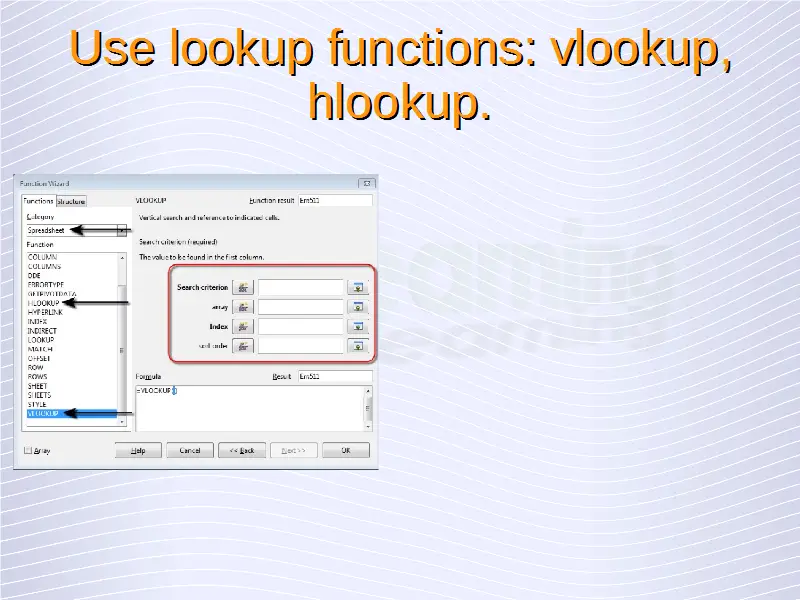
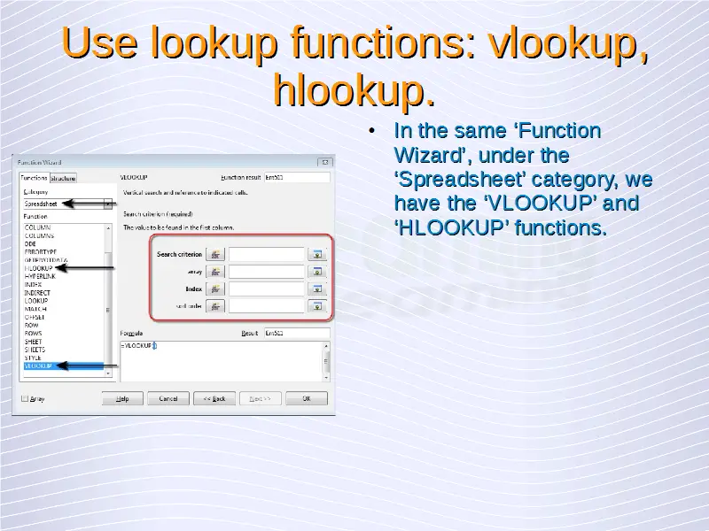
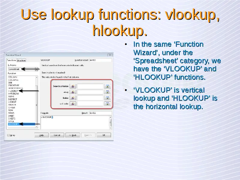
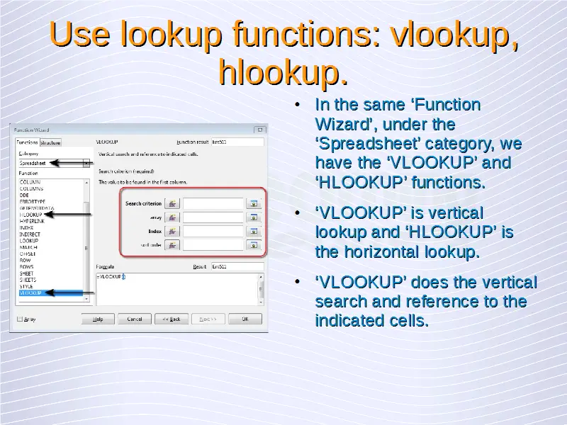
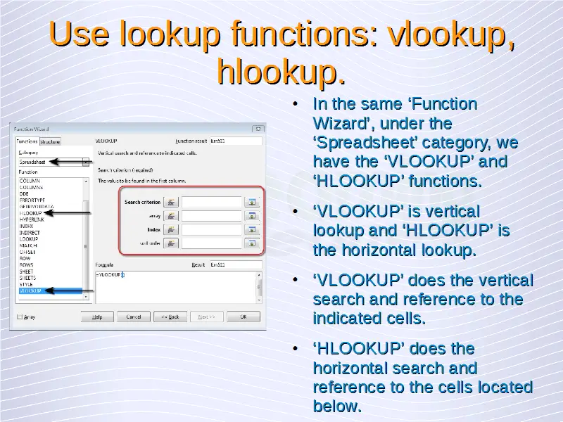
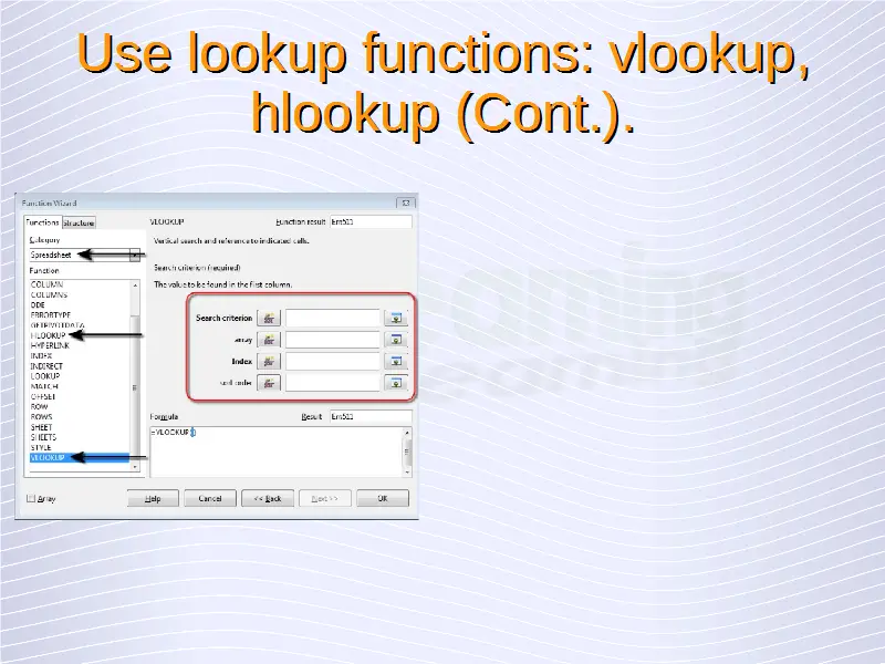
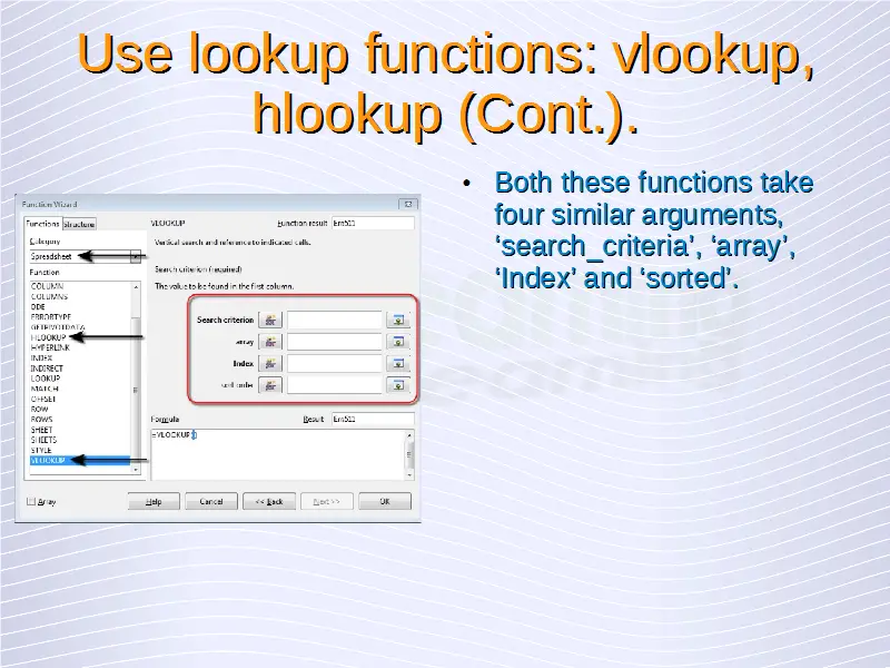
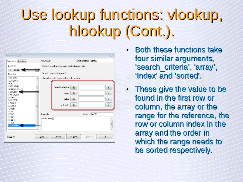
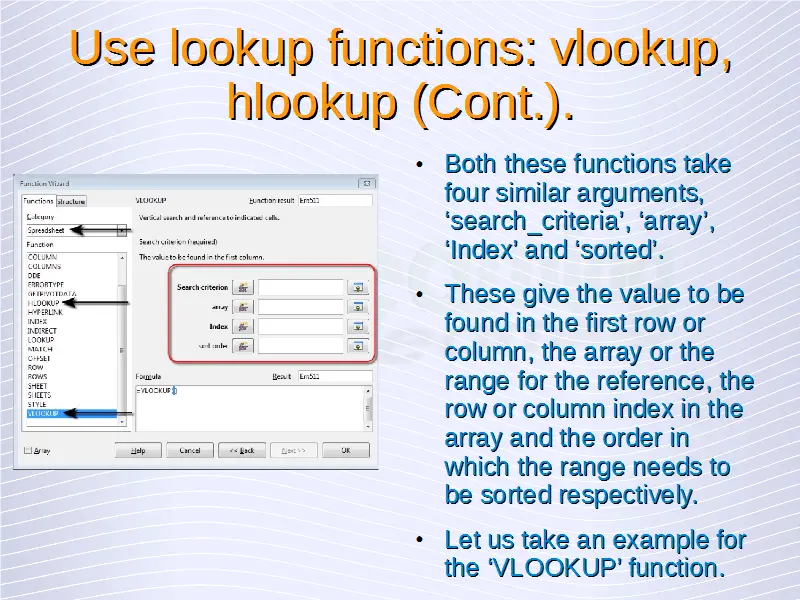
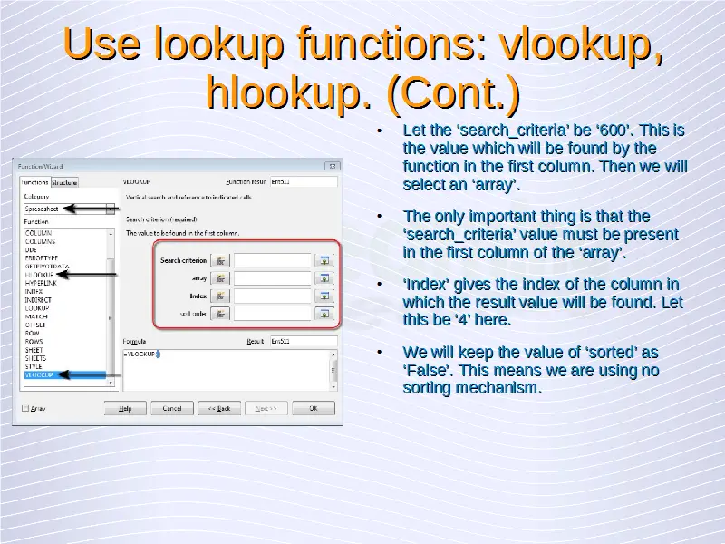
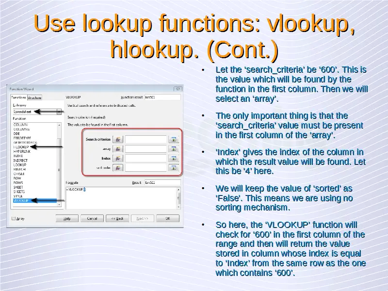
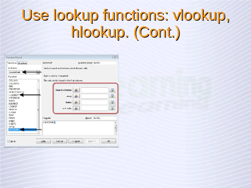
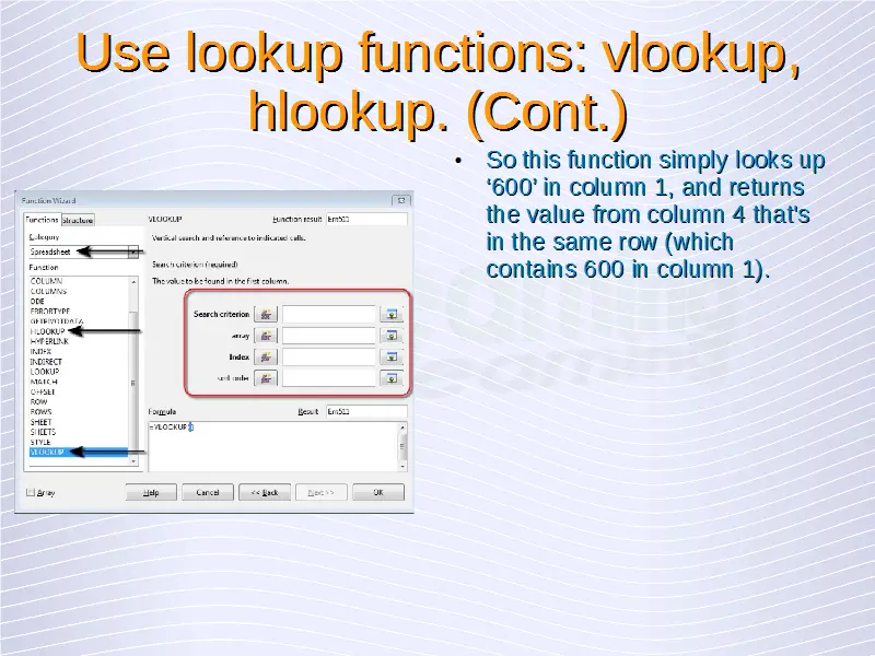
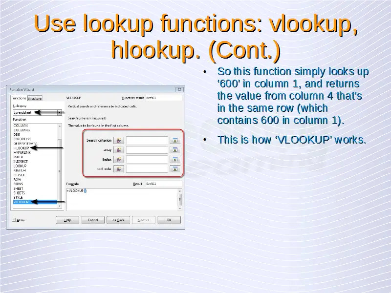
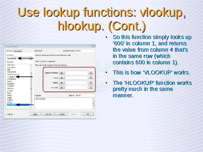
In the same ‘Function Wizard’, under the ‘Spreadsheet’ category, we have the ‘VLOOKUP’ and ‘HLOOKUP’ functions. ‘VLOOKUP’ is vertical lookup and ‘HLOOKUP’ is the horizontal lookup. ‘VLOOKUP’ does the vertical search and references to the indicated cells. ‘HLOOKUP’ does the horizontal search and reference to the cells located below. Both these functions take four similar arguments, ‘search_criteria’, ‘array’, ‘Index’ and ‘sorted’. These give the value to be found in the first row or column, the array or the range for the reference, the row or column index in the array and the order in which the range needs to be sorted respectively. These arguments can be entered either manually or by using the ‘Select’ or ‘Function’ icons.
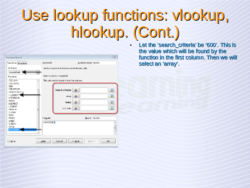
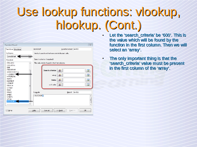
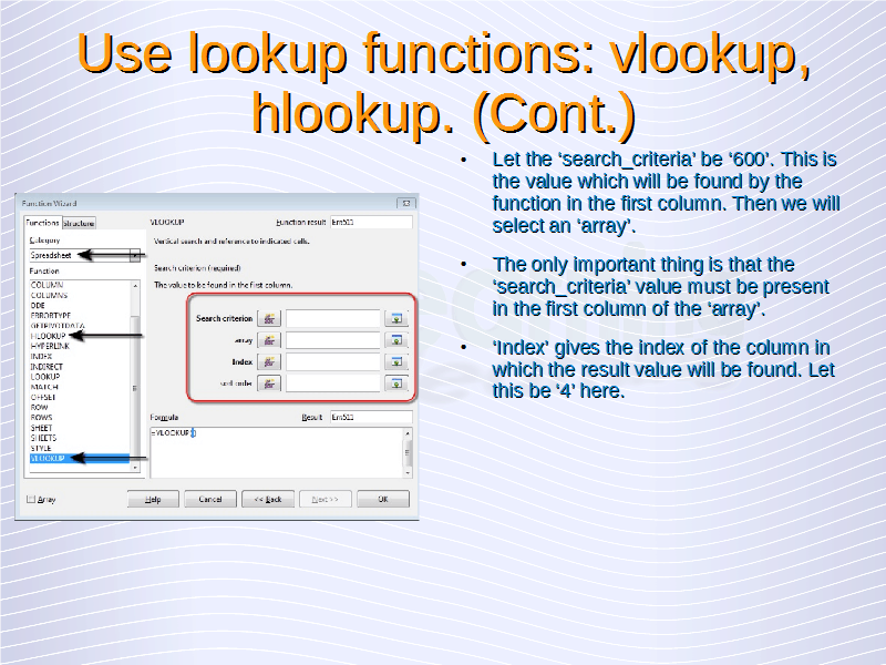
Let us take an example for the ‘VLOOKUP’ function. Let the ‘search_criteria’ be ‘600’. This is the value which will be found by the function in the first column. Then we will select an ‘array’. The only important thing is that the ‘search_criteria’ value must be present in the first column of the ‘array’. ‘Index’ gives the index of the column in which the result value will be found. Let this be ‘4’ here. We will keep the value of ‘sorted’ as ‘False’. This means we are using no sorting mechanism. So here, the ‘VLOOKUP’ function will check for ‘600’ in the first column of the range and then will return the value stored in column whose index is equal to ‘Index’ from the same row as the one which contains ‘600’. So this function simply looks up ‘600’ in column 1, and returns the value from column 4 that’s in the same row (which contains 600 in column 1). This is how ‘VLOOKUP’ works.
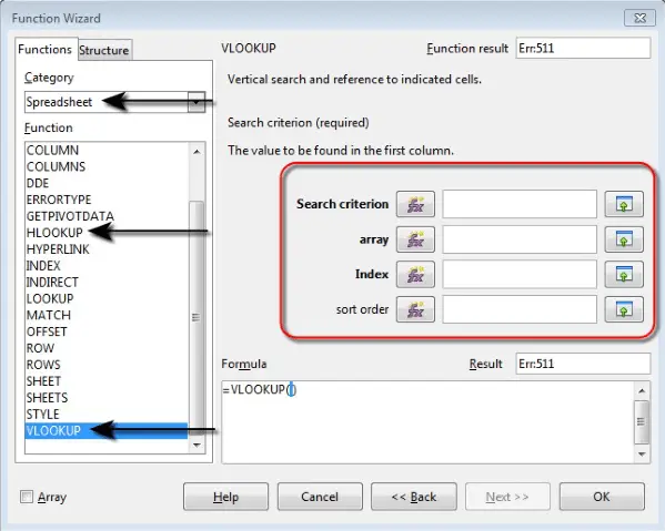
The ‘HLOOKUP’ function works pretty much in the same manner. The only thing is that the ‘search_criteria’ is looked up for in the first row and the value is returned from the row given by ‘Index’ in the same column.

