Apply conditional formatting based on cell content.
Conditional formatting helps us in formatting only those particular cells which satisfy the specified conditions. This means that in any selected cell range, we will define some condition and the cells which satisfy this condition will get formatted while the others will remain as it is.
To apply conditional formatting, first of all make sure that ‘AutoCalculate’ is enabled. This can be checked by clicking ‘Tools’ on the main menu bar.


From the resulting drop-down, click on ‘Cell Contents’, and from the submenu, enable ‘AutoCalculate’.
Now select the data range on which the formatting needs to be applied.


After this, click on ‘Format’ from the main menu bar. From the drop-down, click on ‘Conditional Formatting’, and from the sub-menu select either one of ‘Condition’, ‘Color Scale’ or ‘Data Bar’. All of these will open the ‘Conditional Formatting’ dialog.
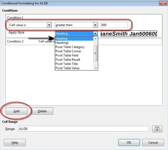


Create the conditions from the options available and then click on ‘Add’ to add the newly created condition. Create as many conditions as required by using different values and color schemes and styles and finally click on ‘OK’ after creating and adding all the required conditions. On click of ‘OK’, the formatting of the cells which satisfy the added conditions will change as per the defined styles.